
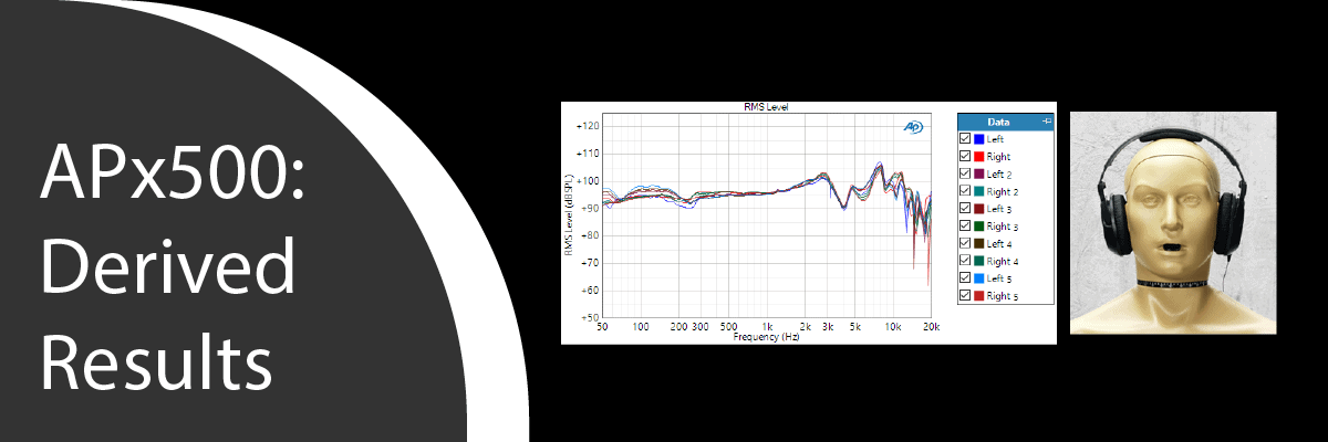
APx500 Tips: Derived Results
In this post, we discuss Derived Results in the APx500 software, another useful feature to help satisfy your audio test needs.
Primary Results in APx are the measurement results that are directly available. The most common types are “Meter” results and “XY” results. Meter results have a single value for each input channel and are represented in APx as a horizontal bar graph – for example, the Gain result in the single-frequency Level and Gain measurement (Figure 1a). XY results display curves of measured values versus an independent variable such as frequency or time – for example, the Gain (versus frequency) result in the Frequency Response measurement (Figure 1b). A third (and less common) result type in APx is the “Tabular” result, which provides a table of values – for example, the Thiele-Small Parameter result in the Impedance measurement. In Sequence Mode measurements, all Primary results are available when a measurement is first added to the project. In Bench Mode, typically only one or two of the most common Primary Results are present, and more can be added, if required.
Figure 1. Examples of a Primary Meter Result (a) and XY Result (b) in the APx500 software
Derived Results are calculated results that can be derived from other measurement results, via math operations such as averaging, smoothing, comparison, normalizing a curve, etc. They can be derived from Primary Results, or from other Derived Results, and they are available in both Sequence Mode and Bench Mode.
To illustrate Derived Results, we’ll use the test case of measuring the frequency response of headphones on a test fixture called a Head and Torso Simulator (HATS). Figure 1 shows RMS Level versus frequency data for five appended measurements of the same pair of headphones on a HATS, with the headphones being removed and replaced on the fixture for each measurement repetition. This procedure, which is a form of “spatial averaging”, is a recommended practice when testing headphones. The measured response varies significantly with the position of the headphones on the fixture due to the interaction of the earphones with the fixture’s pinnae (outer ears). To compensate for this variation, we measure several data sets with the headphones being re-fit on the fixture and then average the results. In addition to spatial averaging, there are other metrics we can calculate from this data set. This is where the Derived Results capability comes into play.
Figure 2. Acoustic response measurements (left) made on a GRAS KEMAR Head and Torso Simulator (right).
The process of adding a Derived Result to a measurement is like most features in APx – there are several ways to get there, including:
- - Right-click on the source result’s graph, on its thumbnail in the Film Strip below the graph, or on the measurement node or source result node in the Navigator, and select Add Derived Result from the context menu.
- - In the measurement’s result view, click on the Add button on the toolbar below the graph and select Derived Result.
- - From the Project menu, select Add Derived Result.
Selecting Add Derived Result opens the Add Derived Result dialog, shown in Figure 3a. In this dialog, the Source control selects or indicates which parent result you wish the new result to be derived from. If you pre-selected the source by right-clicking on a result, this field will be disabled and greyed, as shown in Figure 3. Otherwise, it will be a pulldown menu containing the results in the currently active measurement.
Figure 3. The Add Derived Result dialog, showing (a) the Derived result pulldown menu, and Options sub-menus for (b) Min/Max Statistics, (c) Normalize/Invert, (d) Specify Data Points and (e) Smooth.
The Derived control in the Add Derived Result dialog is a pulldown menu containing a list of Derived Results that can be derived from the selected Source result. This list is context sensitive. For example, the Smooth derived result is available for an XY Source result, but not for a Meter result. Some Derived Results, when selected, present an additional menu in the Options box. For example, Figures 1 (b) through (e) show the Options presented for Min/Max Statistics, Normalize/Invert, Specify Data Points and Smooth, respectively.
Returning to the headphone measurement data, Figure 4 shows spatial average data for the left and right earphones. In this case a Power Average (XY) derived result has been added, derived from the RMS Level result in Figure 2. The result has two Result Specifications, as shown in Figure 5; one for the trace labeled “Left Avg”, which averages all data sets for Ch1 and one for the “Right Avg” trace, which averages all data sets for Ch2.
Figure 4. Spatial average of 5 measurements for the Left and Right earphones; Power Average results derived from the data in Figure 2.

Figure 5. Derived Result Settings for the Power Average Derived Result in Figure 4, and Result Specification for the Left Avg trace.
An important attribute of higher quality headphones is how well the frequency response of the left and right earphones match. We can easily quantify this by adding a Compare Derived Result derived from the spatial average data sets in Figure 4. This yields the Left/Right Track graph in Figure 6, which indicates, that for these headphones, the left and right earphones are within about ±3 dB from 100 Hz to 8 kHz (a perfect match would yield a flat line at 0 dB). As shown in Figure 7, this result was created by deriving a Compare result which compares the Ch2 averaged curve to the Ch1 averaged curve. Note that the Compare result was derived from a Smooth result, derived in turn from a Power Average result, derived in turn from an RMS Level primary result. Any number of Derived Results can be chained together like this.
Figure 6. Left/Right Track result created using a Compare Derived Result.
Figure 7. Settings for the Compare Derived Result used to create the Left/Right Track result in Figure 6.
Next, let’s consider a Meter Derived Result. Suppose we want a single number to quantify the output of each earphone. We could use a Specify Data Points – Single Value result to get the value of the frequency response curve at a reference frequency like 500 Hz. But, since headphone response curves vary significantly with frequency, it might be more appropriate to consider a power average of the levels over a mid-frequency range – say 500 Hz to 2 kHz, as shown in Figure 8. This result was created by first deriving a Specify Data Points result from the spatial average result in Figure 4, to yield curves of left and right average level within this frequency range. A Min/Max Statistics – Single Value – Power Average result was then derived from this intermediate result to achieve the desired metric.
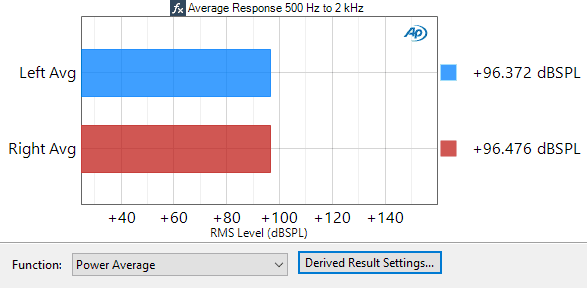
Figure 8. Power averaged response from 500 Hz to 2 kHz.
Derived results are a great tool to help you glean information from your measurement data. Hopefully this brief introduction has provided some insight into how you can use this feature for your audio test projects.

For engineers looking to develop API programs using recent versions of Python, this post will support users in developing those solutions.
Read more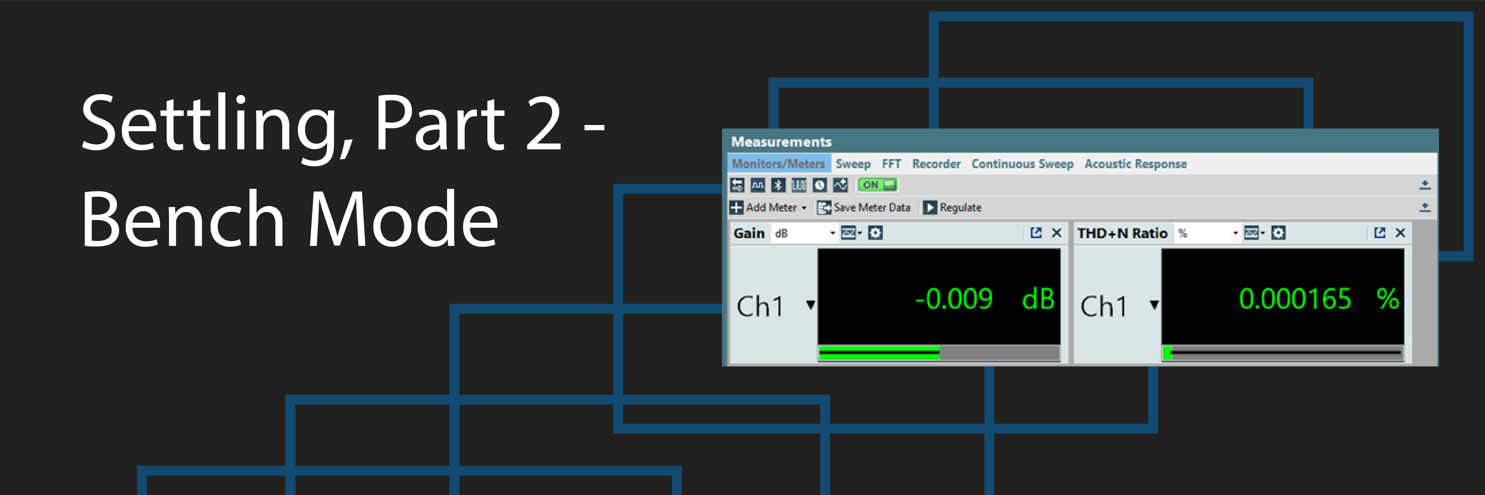
In this two-part series, we’ll review the features available in APx500 software to help ensure that settled readings are acquired when testing audio devices.
Read more
New Video! Mike Martin walks through key loudspeaker test methods, typical test setups and then demonstrates a variety of measurements.
Read more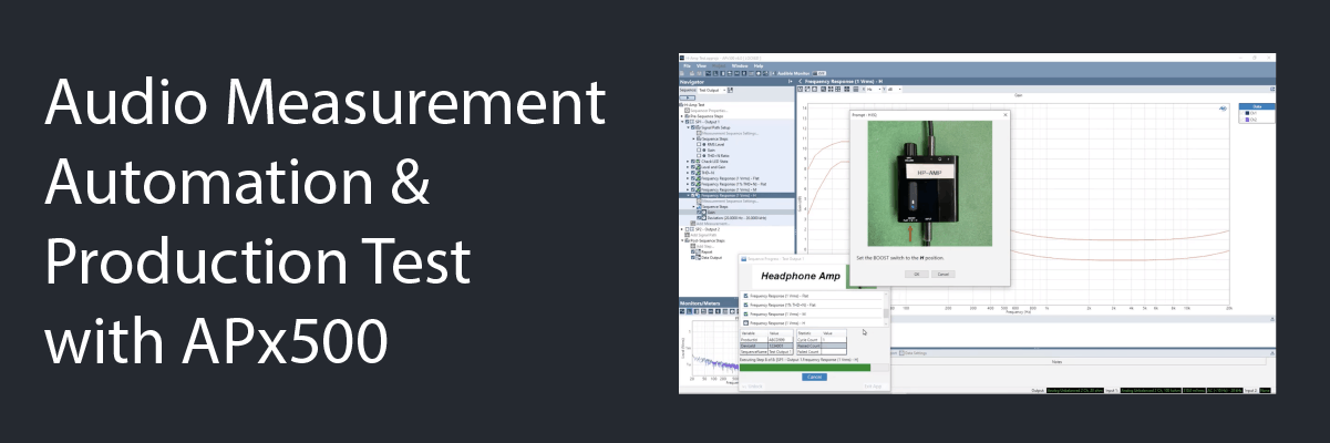
New Video! In this session, Joe Begin provides a detailed discussion of how to use a variety of automation and production (or manufacturing) test-oriented features.
Read more