
Introduction
The APx Polar Plot Utility is a Windows application for making polar measurements of loudspeakers or microphones with an APx500 audio analyzer and for creating 2-dimensional polar dispersion plots from the measured data. The utility, which runs in a small window outside the APx500 software, is used to control a turntable and the connected APx500 Series audio analyzer to automate the collection of polar measurement data. Once the data collection is complete, the utility can be used to create polar dispersion plots.
Requirements
To use the APx Polar Plot utility, a matching version of the APx500 measurement software must be installed on the PC. For example, if APx500 v3.4 is being used, v3.4 of the Polar Plot utility is required.
The APx Polar Plot utility also requires the SPK-RD software option to be installed on the connected APx audio analyzer. If you require a SPK-RD software option, please contact your Audio Precision sales representative.
Note: The Polar Plot Utility will run when the APx500 software is in Demo mode. As such, you can evaluate the utility by creating a Polar project, making measurements using a simulated turntable, and creating a polar plot. There is a restriction, however, in Demo mode: The only data set that can be opened and plotted is the sample polar data set installed with the utility for demonstration purposes.
Polar Angle Convention
This utility uses the following polar coordinate convention: With reference to the face of an analog clock, the zero degree (on-axis) position is at 12 o’clock and angles increase in the counterclockwise (CCW) direction. Some of the turntables supported have a different angular convention. As a result, the angle displayed by the turntable at a given position may be different from the angle displayed by the utility for that same position.
Turntables Supported
The APx Polar Plot utility supports the measurement turntables and control interfaces [1] listed in Table 1. Each turntable is described separately in the Turntable Configuration section.
Table 1. Turntables and interfaces supported
| Turntable |
Supported Interface |
| LinearX LT360EX* |
R/S-232 |
| Outline ET250-3D |
Ethernet |
*Note: *LinearX is no longer in business and the LT360EX Turntable is no longer available. For assistance or support regarding LinearX products, please visit Physical Lab.
Installation
To install the APx Polar Plot utility, run setup.exe in the sub-folder named Volume. The utility application was created using LabVIEW. Therefore, the installer will also install the LabVIEW runtime engine. In addition, it will install the sample polar data set, this instruction document, and any drivers needed to control the supported turntables.
Using the Utility
The Polar Plot Utility has a small user interface window that can be position beside the APx500 UI for convenience. If the corresponding version of APx is already running, the utility will work with it. If APx is not running, the utility will launch it once it is opened.
When the utility is first opened, only a few controls are operable, as shown in Figure 1:
· New Polar Project button – Starts a new polar measurement project
· Open Polar Project button – opens an existing polar measurement project
· Help button – opens the PDF version of this document.
· APx Visible checkbox – toggles the APx UI between visible and invisible states[2].
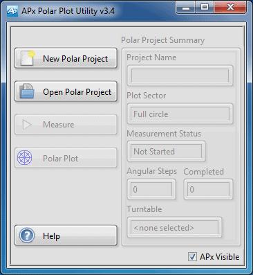
Figure 1. APx Polar Plot Utility window when first opened.
Polar Projects
The utility uses the concept of a polar project, which consists of all the configuration settings for the polar measurements, the turntable used and the polar plot. The utility stores these configuration settings along with the status of the measurements needed to complete the polar plot in an XML file.
When the New Polar Project button is clicked, the utility will first prompt you to select a folder in which to store the polar project and all its data. Navigate to the desired folder and click the Current Folder button (Figure 2).
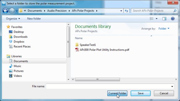
Figure 2. Select folder for new polar project dialog.
Once the folder has been selected, you will be prompted to enter a name for the polar project (Figure 3). As indicated, a folder and file of the same name as the project will be created. Therefore, the polar project name is restricted to valid file naming characters.
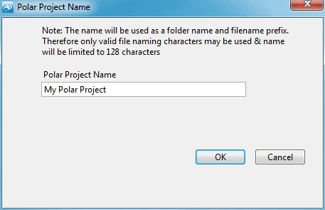
Figure 3. Polar Project Name dialog.
Next, the utility will prompt you to select and configure a turntable (Figure 4). As shown, a simulated turntable is available for demonstration purposes.
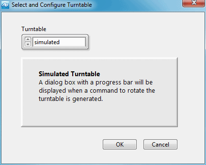
Figure 4. Turntable configuration dialog.
The settings needed to configure the turntables are shown in Figure 5 and discussed separately in the Turntable Configuration section.
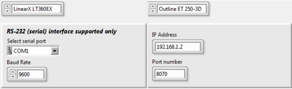
Figure 5. Turntable configuration parameters.
Turntable Configuration
LinearX LT360EX
Support for control via R/S-232 (serial interface) is provided in the utility. This requires a 9-pin straight –through serial cable (one ships with the turntable) and an R/S232 serial port on the PC. Serial ports are becoming less common on PCs; although desktops often have at least one serial port, it is rare to find a modern laptop that has one. One solution for a laptop is to use a port replicator, because these often have a serial port. If none of the above options is available, a USB to R/S-232 converter can typically be used. We tried two different converters (a Digitus USB to Serial Converter and a TRENDnet USB to RS-232 Serial Converter TU-S9) on PCs running Windows 7 and both worked flawlessly on the first attempt with the driver which is automatically installed by Windows. The latter converter was purchase online for less than $10 USD. Note: A windows application that provides complete control of all turntable functions is provided by the manufacturer.
Outline ET250-3D
This is the current turntable offered by Outline Professional Audio of Italy. Support for control via Ethernet is provided in the utility. This requires that the PC and the turntable be on the same network. If the control PC is already on a network, the options are (1) configure the turntable’s IP address to the required subnet and connect it to the same network, or (2) add a second network card to the PC, connect it to the turntable and configure it to be on the same subnet as the turntable. Consult the turntable user manual for instructions to get and set its IP address.
The utility requires that you enter the IP address of the turntable and a port number. If you don’t know the port number, leave it at the default setting. You will have an opportunity to try different port numbers in the subsequent communication test.
An application called ET Commander is available from the manufacturer for controlling all functions of the turntable. This application can be used to debug communication.
Turntable Communication Check
Once the turntable has been selected and configured, the utility will test for proper turntable communication. If communication is successful, it will proceed with creating the polar project. Otherwise, creation of the polar project will be cancelled.
In the case of the LinearX LT360EX and the Outline ET250-3D, the utility simply makes a function call to the turntable to check for a valid communication link. In the case of the Outline ET250-3D with its simpler control interface, the test is not so simple. In this case, the communication test is done during the Turntable Adjustment Step, described below.
Turntable Adjustment Step
Following successful completion of the turntable communication test, the utility presents an adjustment dialog for the LT360 and the ET250-3D turntables, as shown in Figure 6: It displays the current angle, and offers the user a choice of actions to take before beginning (or resuming) a set of polar measurements. These actions are (1) Stay at the current angle, (2) Move to the origin (zero degree position), or (3) Reset the turntable so that the current position becomes the zero degree position.
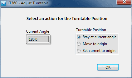
Figure 6. Turntable adjustment dialog (LT360 and ET250-3D).
Configuring Angular Test Position
Following the turntable adjustment step, for a new project, the Configure Angular Test Positions window (Figure 8) opens. This dialog is used to configure the angular measurement and plotting positions. The Measurement Sector control can be used to select from Full Circle, Semi-Circle, ¼-Circle and Custom. The Step Size control can be used to adjust the angle between measurements. The colored round indicator to the left of the Test Positions graph indicates whether the combination of Measurement Sector and Step Size results in an integer number of steps (green) or not (red).
If the Measurement Sector is set to Semi-Circle or ¼-Circle, the Reflect about 0 Axis check box becomes enabled. By checking this box, you can have the utility reflect the data measured from one side of the polar circle to the other, as shown in Figure 8, to take advantage of symmetry.
As the various controls are adjusted, the positions to be measured and plotted are shown in the Test Positions graph and listed in the table to the right of the graph.
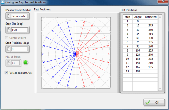
Figure 8. Configure angular test positions dialog.
Conducting Polar Measurements
Once the angular test positions have been configured, the utility’s main window will appear as shown in Figure 9: The Measure button is enabled and so is the Polar Project Summary box, which indicates the state of the project, including Measurement Status, the total number of Angular Steps to be measured, and the number of steps completed.
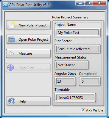
Figure 9. Main window - ready for measurements.
When the Measure button is clicked, the message box in Figure 10 will be displayed. The idea here is to configure one of the several types of frequency response measurements available in APx as required to make the desired measurements, and make it the active measurement, by selecting one of its results (e.g., Level). The utility will then use the same measurement configuration for all of the angular steps included in the polar project. We recommend saving the APx project file once the measurement has been configured, in case the tests are interrupted before all measurements are complete. Supported APx Measurements include Acoustic Response, Frequency Response, Continuous Sweep, Stepped Frequency Sweep, Bandpass Frequency Sweep and Multitone Analyzer.
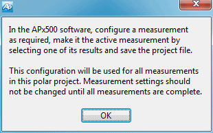
Figure 10. Prompt displayed after Measure button clicked.
Next, the utility executes the “Rotate and Measure Loop” (Figure 11). In this mode, it simply runs the selected APx measurement at each of the selected angular test positions and then rotates the turntable to the next measurement position in a loop, until all measurements are completed, or the operations is cancelled by the user.
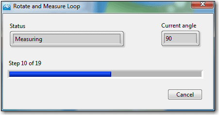
Figure 11. Rotate and Measure Loop dialog.
After each measurement step, the utility saves the measured level response data to an Excel file in the polar project folder, and it also updates the polar project’s xml file. This way, if the measurements are not completed for any reason, you can open the project file at a later time and resume making measurements where you left off. This is another reason that it is important to save the APx project file, to get consistent results.
Making Polar Plots
When the measurements are complete, the utility’s main window will appear as shown in Figure 12: The Measurement Status indicator shows Complete and the Polar Plot button is enabled.
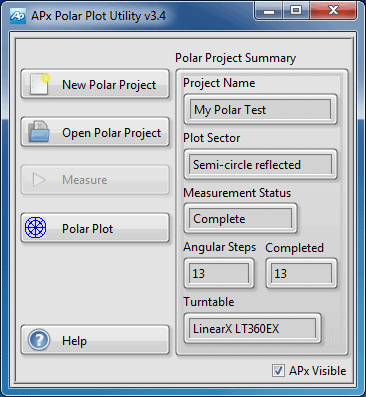
Figure 12. Measurements completed.
It is required to keep the APx500 software open for polar plotting, because the utility uses features built into APx500 to smooth the response data and to decimate the frequencies to IEC preferred 1/n-octave smoothing. When the Polar Plot button is clicked, the utility will launch the Polar Plot Response Data window (Figure 13). It will also process the response data by importing the measured level response curves into a temporary measurement in APx and using derived results to smooth and decimate the frequency response data.
The following controls and indicators are available on the Polar Plot window.
| Position knob | Used to select an angular position. |
| Response at Selected Position | Graph showing the frequency response for the currently selected angle. |
| Cursor on Response Graph or
Frequency control on Polar Plot |
Dragging the cursor changes the selected frequency and updates the polar plot. Alternatively, you can change the frequency using the control in the upper left corner of the poplar plot. |
| Visible Section | Can be used to change the portion of the polar plot displayed (full circle, semi-circle, quadrant, etc. |
| Wrap | If checked, joins the first and last points measured (checked by default when a full circle is being displayed). |
| Normalize | If checked, displays the response magnitude relative to the on-axis response; otherwise displays the absolute level in dB units (checked by default). |
| Smoothing | Used to select the level of smoothing (from 1/1 to 1/24-octave or None). This control causes the data to be reprocessed in APx. |
| Decimation | Used to select the frequency decimation (from 1/1 to 1/24-octave or None). This control causes the data to be reprocessed in APx. |
| Save Image | Used to save an image of the polar plot as a .png file. |
| Multiplot | Invokes the polar multiplot window. |
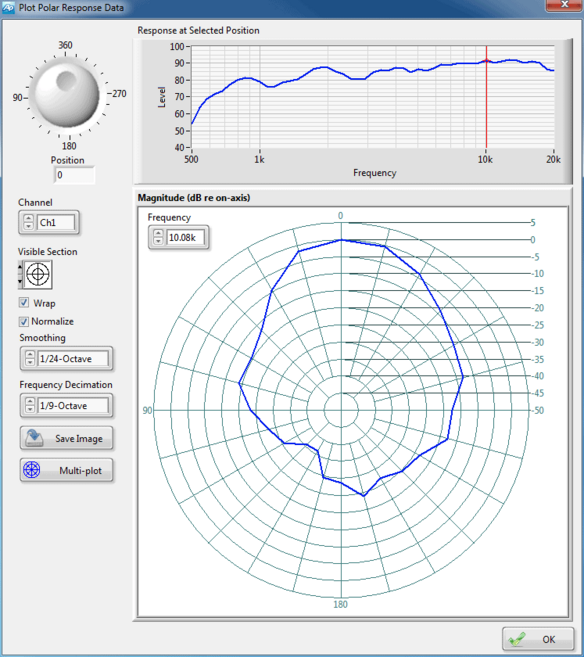
Figure 13. Polar Plot window.
Polar Multiplot
The polar multiplot window is shown in Figure 14. It displays polar plots for up to 6 frequencies on the same graph simultaneously.
Figure 14. Polar multiplot window.
To hide a trace, simply uncheck the check box beside it in the legend. The Directivity table will automatically be updated to correspond to the displayed traces. You can also change the frequency of a trace by typing the desired frequency in the control beside the trace in the legend. To change the color of a trace, click on the trace in the legend and select a different color. The Line Width control can be used to change the line width of all the traces displayed. The Save Image control can be used to save a .png file of the polar multiplot including the directivity table.
[1] . Each turntable has other control options than those listed, but currently, only the interface listed in Table 1 is supported.
[2] Note: If you make the APx UI invisible and then close the utility, the APx500 software will still be running in the background. To close it, you can run the utility again, make APx visible and shut it down normally, or you could end the program while it’s still invisible using Task Manager.
All product and company names are trademarks™ or registered® trademarks of their respective holders. Use of them does not imply any affiliation with, or endorsement by, said organizations.
RELATED DOWNLOADS