
Measurements are Estimates
“Measurements are estimates” is a phrase an old boss of mine would use. I think this phrase is incredibly useful in the context of audio test because it helps to frame the way we approach making measurements. Instead of thinking of audio analyzers as returning absolute truths, we should think of them as tools for estimating various properties of sound. Once we understand that we have a device that makes estimates, we can start thinking about what affects the accuracy of those estimates.
First and foremost, audio analyzers are not perfect devices. They are real-world machines with their own residual noise and distortion, frequency response, and so on. For example, when you estimate the noise of a device by measuring it with an Audio Precision audio analyzer, you are measuring the sum of the noise of the device under test (DUT) with the self-noise of the instrument. These add as the root of the sum of the squares of the two values. This can be useful to get a closer estimate of the DUT noise by measuring the analyzer residual noise with no DUT connected, then measuring the DUT noise with the analyzer, and finally solving the equation for the DUT noise using the formula DUT noise = square root of the (Total Noise)2 minus the (Analyzer Noise)2.
The reason the analog performance of AP analyzers is so critical is that if you are very close to the residual or intrinsic performance of the instrument, the inherent resolution of the instrument will limit the accuracy of your estimate. As a rule of thumb, when measuring noise or distortion you would like the analyzer to have a residual on the order of 10 dB lower than the device being measured.
A second idea that is introduced by thinking of measurements as estimates is that in some cases, the more time we spend making an estimate, the more accurate it is likely to be. In our day-to-day life, if you want to measure a distance very accurately it takes some care to do so. In audio measurement, where we are inherently characterizing a time varying signal, this applies in several ways.
If we are estimating the level of a noise, that is we are trying to approximate the value of a constantly varying signal then intrinsically the longer we sample that signal for, the more accurate our measurement will be.
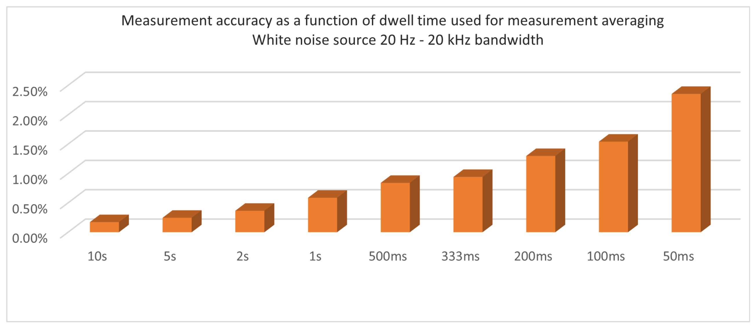
In the graph above we are looking at the measurement accuracy in estimating the amplitude of a white noise source over a 20 Hz to 20 kHz bandwidth. If you average the signal for just 50 ms, the accuracy is just over 2%. If you have the patience to average it for 10 seconds, the accuracy becomes 0.2%.
In other measurement contexts, additional measurement time can be used to reduce the effects of noise. For example, when performing Fourier analysis you can average acquisitions in the time domain (i.e., synchronous averaging). As a general rule for uncorrelated noise components, the S/N ratio improves by the Square Root of N where N is the number of averages performed.
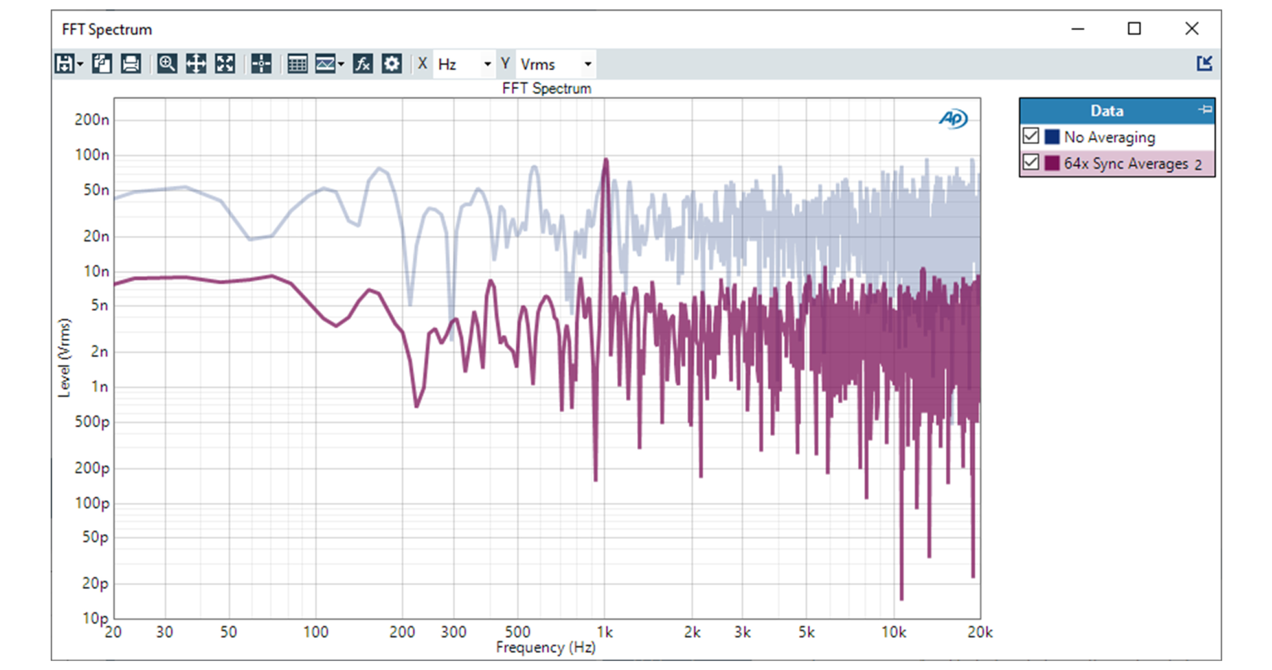
In the above graph, we are trying to resolve a very small signal. Without any averaging the signal can’t be discerned from noise, but after 64 synchronous averages, the random noise is reduced and the coherent signal can be very accurately measured.
That is, while we would normally believe that the only way to improve signal-to-noise ratio in a measurement is to increase the signal level or decrease the noise, there is a third option. Where the signal includes uncorrelated noise, averaging increases the amount of time we dwell on a measurement, but that time results in a better signal to noise ratio and better measurement accuracy.
Measurements are estimates; the more care we take in making an estimate the more accurate our measurements will be.
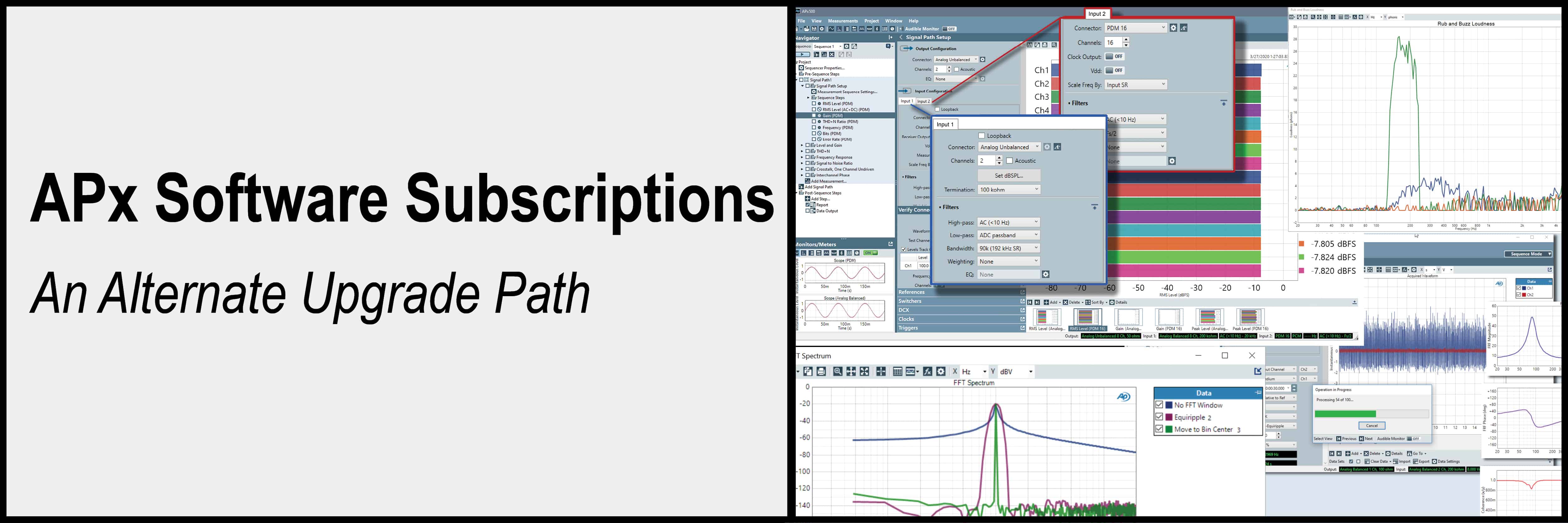
Introducing a new way to access all the latest APx500 software versions
Read more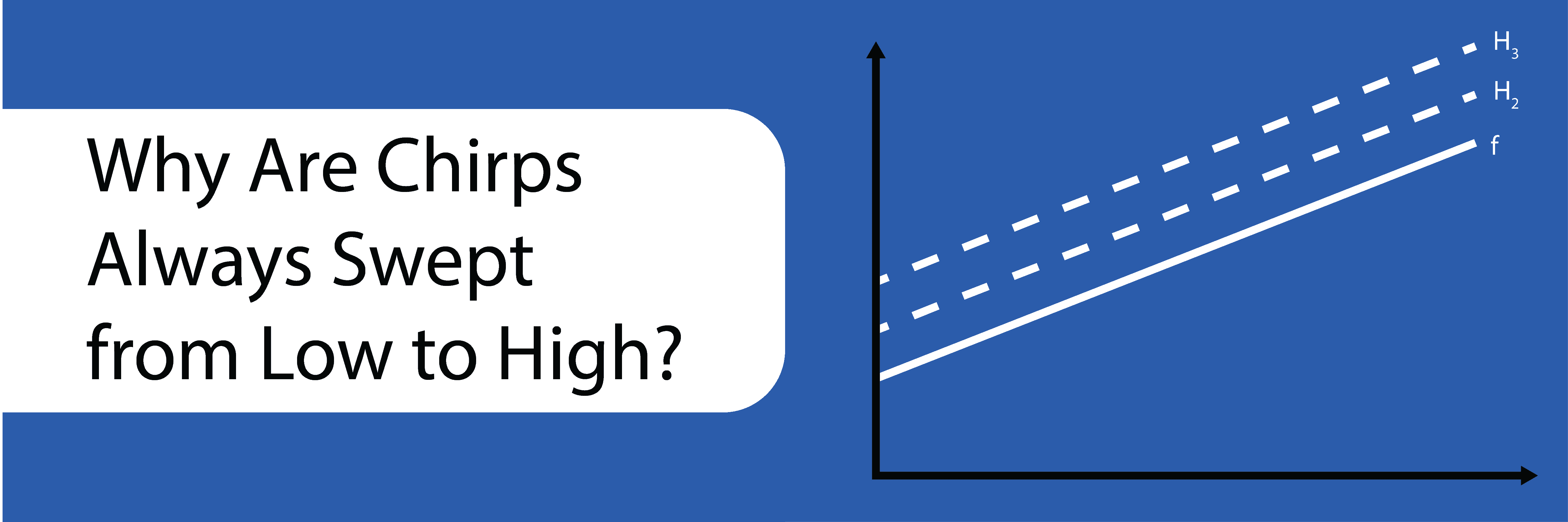
If you look at any APx measurement using a log-swept sine stimulus (a chirp), you might notice that the signal is always swept from low to high frequency. Learn more about why chirps are always swept from low to high.
Read more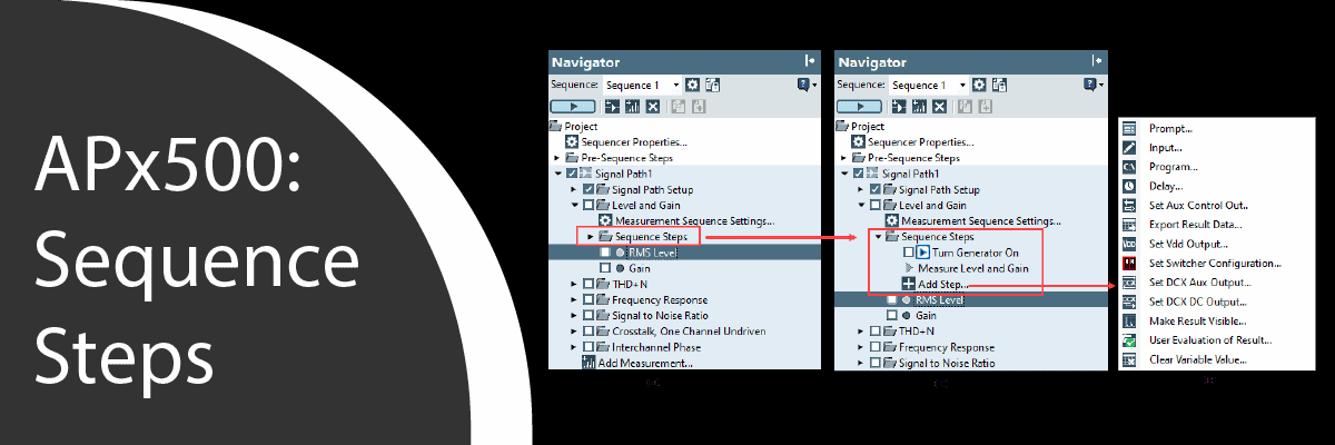
With its built-in test sequencer, reporting engine, and more, Sequence Mode in APx500 software can be very useful for a variety of applications.
Read more
Benchmarks. They are vital to ensure the R&D team produce a compelling new product or service and are essential on the production line of a manufacturing facility.
Read more