FFT Spectrum and Spectral Densities – Same Data, Different Scaling

Fast Fourier Transform (FFT) analysis, which converts signals from the time domain to their frequency domain equivalent, is incredibly useful in audio test. Precise estimates of many fundamental audio quality metrics such as frequency, level, harmonic distortion, intermodulation distortion, crosstalk, etc., can all be derived from FFT analysis. In fact, all but a few of the hundreds of results available in Sequence Mode in the APx500 software are derived from FFT analysis.

Most users are familiar with the FFT Spectrum result, typically used for analyzing signals with discrete frequency components (like sine waves). But many may be less familiar with the Power Spectral Density and Amplitude Spectral Density results, which are typically used when analyzing noise. This post explains the difference between these spectral density results and the more commonly used FFT Spectrum.

FFT Spectrum

For illustration purposes, Figure 1 shows a signal that contains both a discrete frequency component as well as a relatively high level of broad band noise. The noise was created by using a digital interface with dither applied at a bit depth of only 8 bits. The Scope (waveform, left) and the FFT Spectrum results (right) for this sine signal at 1125 Hz with a level of -20 dBFS (or 0.10 FS) are shown.

Figure 1. Waveform and 16k FFT Spectrum of a 48 kHz Fs digital sine signal with 8-bit dither (level = -20 dBFS; frequency = 1125 Hz).

The FFT Spectrum result (sometimes called the linear spectrum or rms spectrum) is derived from the FFT auto-spectrum, with the spectrum being scaled to represent the rms level at each frequency. As a result, the FFT Spectrum of a pure sine contains a peak at the frequency of the sine signal with amplitude equal to its rms level. For example, the peak in the FFT Spectrum in Figure 1 is exactly the expected signal level of -20 dBFS. The FFT Spectrum is ideally suited to analyzing signals with discrete components or tones.

But what if we’re interested in quantifying the level of noise in this signal? From a casual observation of the spectrum in Figure 1, we might be tempted to say that “the noise floor in this measurement is at -80 dBFS”, or “the signal-to-noise ratio is 60 dB”. But these statements are wrong, because of the FFT spectrum’s scaling for pure tones. This is obvious when you consider Figure 2, which shows the same signal as Figure 1 analyzed with three different FFT Length settings: 256, 16k and 1M points. Note that the peak remains at -20 dBFS, but the level of the apparent noise plateau decreases substantially as the number of FFT bins is increased.

Figure 2. Linear FFT Spectra of the signal in Figure 1 with FFT Lengths of 256 (left), 16k (middle) and 1M samples (right). Note how the amplitude of the peak at 1125 Hz is constant, but the apparent noise plateau is reduced in level as the FFT Length increases.

The change in level of the noise plateau in Figure 2 is a result of the change in the FFT bin width. The noise is distributed over the entire frequency range, so the wider the FFT bins , the more noise each bin will contain. In fact, each time the bin width is doubled, the noise power per bin is also doubled, causing an increase of 3 dB in the rms level. With smoothing applied to the spectra in Figure 2, the apparent noise plateau is at -62, -80 and -98 dBFS for the FFT Length settings of 256, 16k and 1M, respectively (i.e., a change of -18 dB for each of the two steps). The increases in FFT Length from 256 to 16k and from 16k to 1M each correspond to the FFT bin width decreasing by a factor of 64, or 2^6. As a result, the rms noise level per bin decreases by 18 dB (i.e., 6 x 3 dB) in each case.

Spectral Density Results

The Power Spectral Density is also derived from the FFT auto-spectrum, but it is scaled to correctly display the density of noise power (level squared in the signal), equivalent to the noise power at each frequency measured with a filter exactly 1 Hz wide. It has units of V²/Hz in the analog domain and FS²/Hz in the digital domain.

Figure 3 shows the Power Spectral Density results corresponding to the data of Figure 2. Note that the apparent noise plateau of the signal remains constant as the FFT bin width changes - however, the level of the discrete peak at 1125 Hz does change with FFT Length. In this case, a statement to the effect that “the noise floor in this signal is approximately 1 nV²/Hz” is correct.

Figure 3. The same data as Figure 3 expressed as Power Spectral Density plots. Note how the noise plateau is constant, but the level of the peak increases with the FFT Length.

The Amplitude Spectral Density is also used to analyze noise signals. It has units of V/√ Hz  in the analog domain and

FS/√ Hz in the digital domain. The Amplitude Spectral Density is simply the square root of the Power Spectral Density.

FFT Windows and the Equivalent Noise Bandwidth (ENBW)

When conducting FFT analysis, typically, a window function is applied to the data before taking the Fourier transform to enforce the necessary condition that the signal is periodic within the sampled time block. Many types of FFT windows exist, and each has unique characteristics that offer certain application-dependent advantages and disadvantages. The default window used in APx500 software is the AP Equiripple window. Other common windows include the Hann and the Flat Top window.

A consequence of using an FFT window is that it spreads signal energy from each FFT bin into adjacent bins, effectively increasing the FFT bin width. The relative increase in bin width is characterized by a property known as the equivalent noise bandwidth (ENBW). Each window has a specific ENBW, which must be accounted for when scaling the FFT spectrum. For example, the ENBW of the AP Equiripple and Hann windows are 2.63 and 1.5, respectively. If no window is selected (sometimes called a Rectangular window), the ENBW is equal to 1.0.

The FFT Spectrum and the Power Spectral Density are related by the ENBW as shown in equation (1).

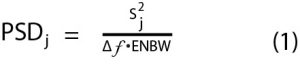
Where PSD represents the power spectral density, S represents the rms (or linear) spectrum, j is the FFT bin number and Δf is the FFT bin width.

Level Calculations

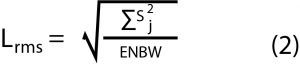
It’s often required to calculate the rms level of noise within a specified frequency range. This can be done by integrating the FFT Spectrum or PSD between the frequencies of interest. Another common requirement is to estimate the rms level of a discrete frequency component, such as a harmonic. Typically, this is done by integrating the FFT over 3 FFT bins on either side of the bin containing the frequency of interest, to account for the spreading effect of the window. Equations (2) and (3) can be used to calculate rms level from the FFT Spectrum and PSD, where each summation is applied over the FFT bins spanning the frequency range of interest.

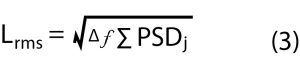
An advantage of using the PSD for this calculation (equation 3) is that it’s not required to know which FFT window was used, because the ENBW is built into the PSD’s scaling.

Reference

Heinzel, G., Rüdiger, A., & Schilling, R. (2002). Spectrum and spectral density estimation by the Discrete Fourier transform (DFT), including a comprehensive list of window functions and some new at-top windows.